Analytics methods

Alongside the physics models of the Digital twin, Tipspeed derives a set of diagnostics from operational data and from satellite imagery. They quantify how each turbine is oriented, how much production is lost and why, and how the turbines actually perform compared to their reference power curve.

Nacelle direction offsets to North

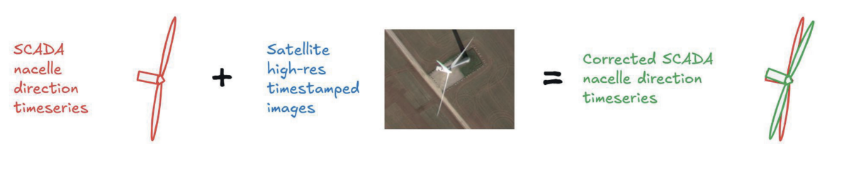
Nacelle direction offsets to geographic North are determined with a patent-pending method based on satellite imagery. It yields the true nacelle direction, which is what makes an absolute yaw misalignment estimate possible.

Workflow for determining nacelle direction offsets to geographic North using high-resolution satellite imagery.

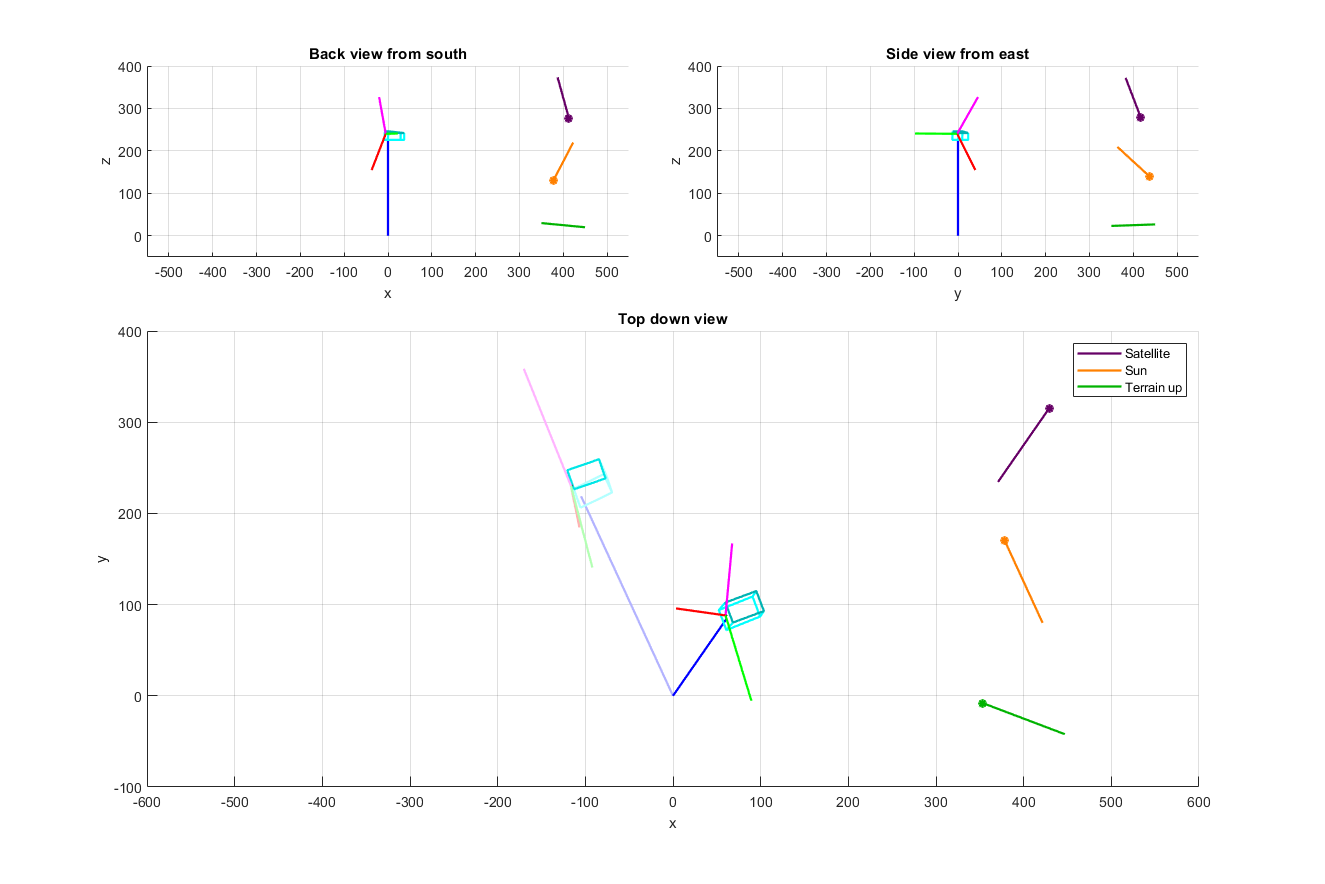
The method builds on a 3D turbine and terrain-specific model that predicts the ground-shadow geometry for any sun and satellite position. The model includes nacelle, blades and tower, parameterised by rotor diameter, hub height, tilt and cone angles, and projects them accounting for sun and satellite positions, terrain slope, nacelle direction and rotor position.

Side and top views of the turbine projection model used to determine the nacelle direction offset.

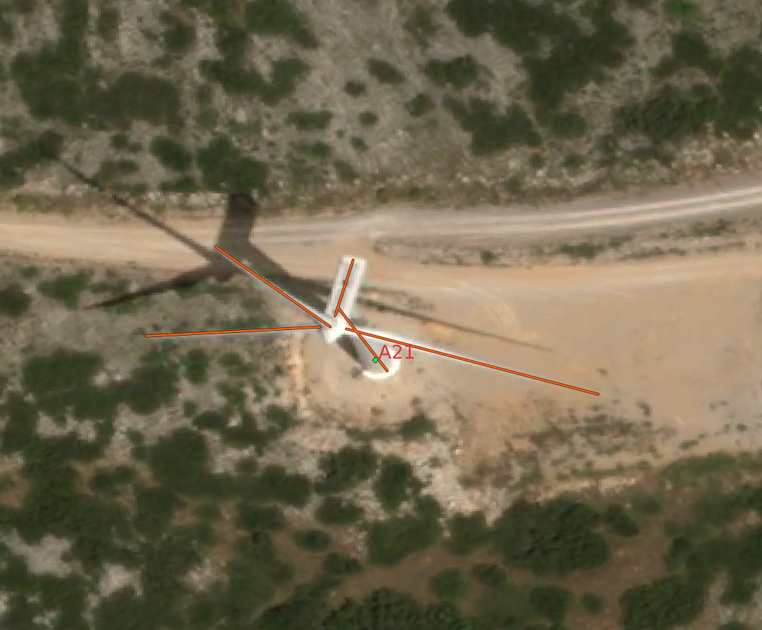
High-resolution satellite imagery is then used to identify the positions of the tower, blade and nacelle, and of their shadows. Estimates of the true nacelle direction are obtained by minimising the error between the predicted and the observed features, and a goodness-of-fit metric discards images whose marked positions deviate significantly from expectations. Experience shows that at least three images per turbine are needed for good accuracy. Further details on the method are given in (Tipspeed, 2025a).

Close-up of a high-resolution satellite image acquired for a site, with marked positions for the tower, blade, nacelle and their shadows.

Once the true nacelle directions are known, offsets to North are obtained by minimising the deviation between them and the SCADA nacelle directions.

Yaw misalignment estimation

Yaw misalignment — the average difference between the orientation of the rotor and the wind direction — causes underperformance. Existing techniques for evaluating it are not fully satisfactory:

• external sensors such as lidar are very accurate but hard to scale;
• SCADA-based analytics do not perform equally well on all turbine types and sites, and depend heavily on input data quality.

Tipspeed has developed a sensor-free method that improves on data-driven techniques by combining high-resolution satellite imagery with numerical weather models (Tipspeed, 2025b). For each turbine, the yaw misalignment time series is the difference between:

• the nacelle direction, corrected for the North offset above;
• the wind direction, corrected by the wind flow model and the wake model.

The method was validated through 19 blind tests with several customers, across six sites on two continents, covering varied terrain complexity and turbine models. All turbines had previously been tested with a nacelle-mounted lidar; the lidar results were disclosed only after Tipspeed had produced its estimates.

Validation of yaw misalignment offsets determined from satellite imagery, against nacelle-mounted lidar.

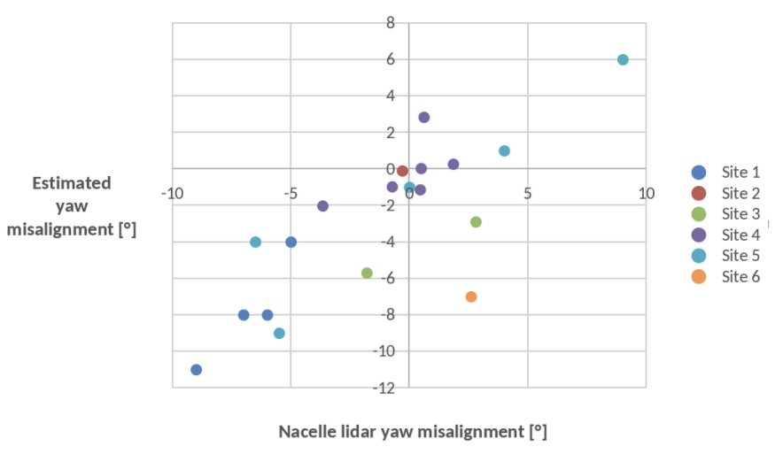
Results show a good correlation and a 2.25° uncertainty (mean absolute error) relative to lidar. One site showed a larger deviation, which is being investigated. On two of the sites, the method was also shown to detect changes of yaw misalignment within a few days.

Restricting the analysis to a power band

Yaw misalignment is not a single number per turbine: it can differ between partial load and rated power. The dashboard's yaw panel therefore accepts an optional power band in kW. When one is set, only 10-minute records whose SCADA power falls in the band — at or above the lower bound and below the upper — enter the average. Records with no power reading are excluded, since they cannot be shown to belong to the band.

The band applies to the misalignment chart, to the per-turbine misalignment column beneath it, and to each turbine's own misalignment scatter, so every misalignment figure on the panel describes the same set of records. It deliberately does not apply to the yaw energy loss, which is a step of the energy chain and must keep reconciling with it, nor to the optimal yaw offset, whose fit defines its own operating window (see below), nor to the headline yaw misalignment figure on the project summary or the map's alignment colouring, both of which describe the turbine's whole operating range rather than one slice of it.

Comparing two groups of turbines

The panel can also split the selected turbines into two groups, A and B, and plot a mean misalignment line for each instead of one site line. A turbine belongs to at most one group. This compares, for example, machines whose nacelle calibration has been corrected against those still awaiting it, over identical periods and — where a band is set — identical operating conditions. The per-turbine table below the chart continues to describe every selected turbine, whether or not it belongs to a group.

Optimal yaw offset

Yaw misalignment estimation, above, measures where the rotor points relative to the wind. It does not say where it should point. The two are not the same: the direction that maximises a turbine's power may differ from the hub-height wind direction. Wind shear, an inclined flow and a wind direction that veers across the rotor all mean the turbine faces more than one wind at once, so the orientation that produces most is not simply the one facing the wind at hub height. Wakes from upstream turbines shift that optimum further. And because the rotor turns one way, a misalignment to the left of the wind does not load the machine, or cost it, the same as the same angle to the right. The optimal yaw offset is the misalignment at which the turbine actually produces most — the target a yaw recalibration should aim at, rather than zero.

We estimate it per turbine, from SCADA alone, in four steps.

Operating window. Only full-performance records between 20% and 80% of the turbine's rated power are used. Above that band the turbine is power-limited and its output stops responding to yaw, so misaligned samples would look indistinguishable from aligned ones; below it the signal is lost in noise.

Reference power. A turbine's power varies far more with the wind than with its own yaw, so the wind has to be removed before any yaw effect is visible. Neighbouring turbines are selected as references — nearby ones first, then those whose power correlates best with the target — and a gradient-boosted regression predicts the target turbine's power from the references' power, nacelle wind speed, blade pitch, rotor speed and orientation. The ratio of measured to expected power then carries the target's own behaviour with the shared resource divided out.

Binning. That ratio is averaged in bins of measured misalignment, each bin keeping its standard error so the fit can weight a well-populated bin above a sparse one. Two binning schemes are computed, one of fixed width and one of equal sample count. They are not averaged: they exist to be compared, and a material disagreement between them is reported as a caveat rather than hidden.

Fit. A cosine response is fitted to the binned means by weighted least squares — power falling as the cosine of the angle away from an unknown optimum, raised to an exponent that the fit also recovers, since real turbines lose power faster than a plain cosine. The location of that peak is the optimal yaw offset, and its uncertainty comes from the fit covariance.

A fit lands in one of three situations. When the curve is bracketed by real observations on both sides, its peak is the optimal yaw offset and is reported as a measurement. When it is not — the peak falling outside the measured range, or barely inside it — the binned response is searched for a discrete peak on the same side of zero as the fitted optimum: a bin whose mean lies above both of its neighbours. Where one exists, the highest such peak is reported instead, carrying the rejected fit's own uncertainty, and the fitted curve is not drawn, because the selection was discrete rather than continuous. Where none exists, nothing is reported: the value is drawn in grey for reference and labelled as having no fit behind it.

Weaker concerns — a wide confidence interval, the two binning schemes disagreeing, the curve shape reaching the limit of its range — are reported alongside the value instead of suppressing it, so a reader can judge how much weight it carries.

The offset that would bring a turbine's mean misalignment to zero is drawn alongside the fitted optimum, so the two candidate corrections can be compared directly. It carries a band of the misalignment's own 2.25° uncertainty, since the figure it is derived from is an estimate rather than an exact angle.

Illustrative. Each marker is one bin of measured misalignment, sized by how many records it holds and carrying its standard error; the curve is the weighted cosine fit through them. The optimum γ₀ is marked with its uncertainty, and the offset that would bring the turbine's mean misalignment to zero is drawn alongside it for comparison.

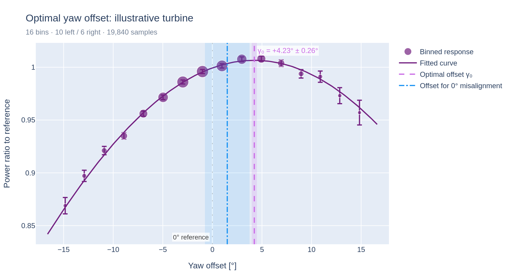
The optimal yaw offset has limits, and on some turbine technologies it is less reliable than on others. It is an informative metric rather than a verdict, and it need not agree with the yaw misalignment derived from satellite observations, which does not depend on turbine technology. Where the two agree — in direction above all — they reinforce each other, and the conclusion carries more weight. Where they disagree, both should be read with more caution.

Expected power

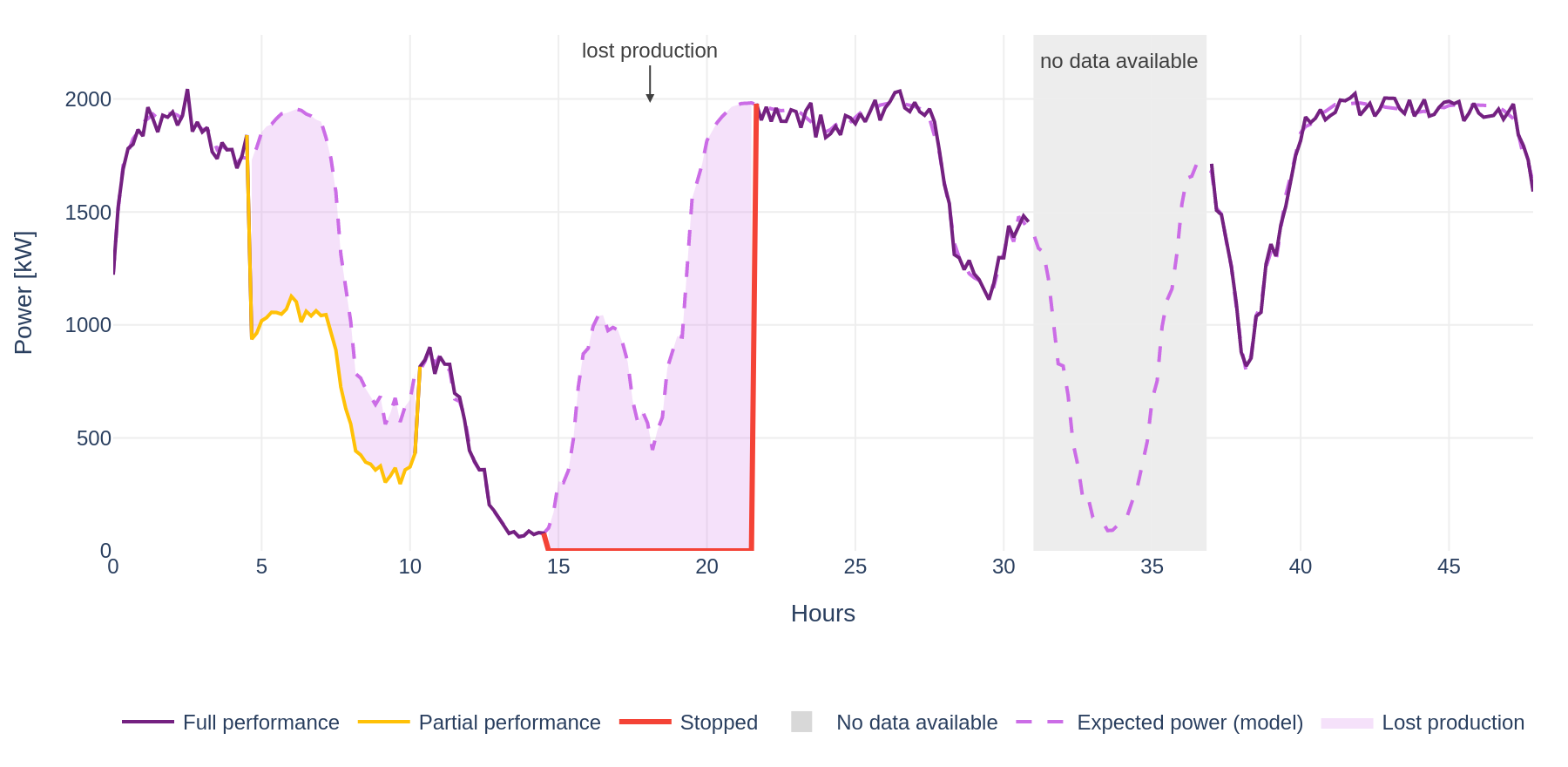
Availability, curtailment and partial-performance losses are all evaluated by comparing what a turbine produced against what it would have produced. That second half is reported nowhere, so it has to be estimated: an expected power series, for every turbine and every 10-minute step, including the steps where the turbine was stopped, was curtailed, or simply did not report. It fills the gaps in the SCADA record, and it is the reference each turbine's production losses are measured against.

Building the expected power series. Each cell is one turbine at one 10-minute step: only the full-performance records teach the model what the turbine can do, and the derated, stopped and absent ones are what it has to fill in.

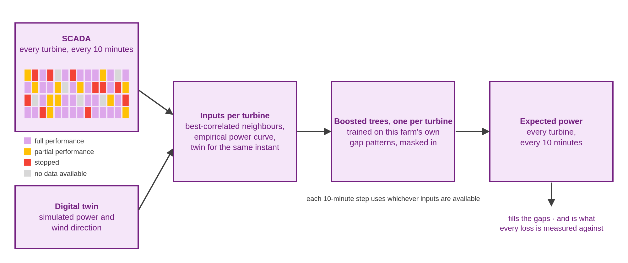
The method rests on the fact that the turbines of one farm see closely related wind. For each turbine, the neighbours whose production tracks it most closely are selected as references. A model then learns to predict that turbine's power from three things: the references' power and orientation, the digital twin's simulated power and wind direction for the same instant, and the turbine's own empirical power curve, fitted from its recent history and corrected for air density. The model is a gradient-boosted ensemble of decision trees (XGBoost), fitted per turbine on that turbine's own full-performance history, so each one learns the behaviour of the machine it describes rather than a farm average.

Data can be missing in several ways: one variable of one turbine, a turbine as a whole, or the whole farm at once. The model is trained to be robust to each of them — part of its training records have inputs deliberately hidden, reproducing the patterns of absence it will meet in production — so the estimate degrades gradually as data disappears rather than failing outright.

A turbine that has not reported for long enough cannot be fitted on its own history. Rather than leaving it out, its model is fitted on the pooled records of the healthy turbines that most resemble it, with every input expressed relative to each turbine's own neighbours rather than in absolute terms, so that the borrowed fit applies to the turbine that lacks history.

A part of the record is held back chronologically and never shown to the model during training. The fitted model is scored on it turbine by turbine, and separately for each pattern of missing data, against the digital twin alone as the baseline to beat. The same scores are computed period by period, so a model that no longer describes a turbine — after a retrofit, a controller change, or a sensor drift — shows up as a trend rather than as a silent error.

What a timestamp means

A time value means different things depending on what it stamps:

• A 10-minute record's timestamp marks the end of the interval it covers: 10:20 covers what happened between 10:10 and 10:20, following the convention of most data loggers and SCADA systems.
• Every aggregated period — hourly, daily and monthly — is labelled by its start instead: the hour 10:00 covers 10:00–11:00 and collects the six 10-minute records 10:10 through 11:00; the day 2026-01-01 collects 00:10 through the next day's 00:00.

Lost production estimation

Production losses are calculated with a power-based lost production estimation method, as recommended by IEC 61400-26 (IEC, 2019). At each 10-minute step, the loss is the expected power minus the power actually produced — never counted as a gain when the turbine outperforms the estimate — attributed to the state the turbine was in at that moment: stopped, partially performing, outside its environmental specification, or not reporting at all. No loss is attributed while a turbine is in full performance: a turbine that runs but under-produces is accounted for earlier in the energy chain, against the digital twin rather than against this series. Summed over a period, those losses become the energy each cause cost, and the same expected series summed over the whole period is the reference they are expressed as a percentage of — the production the farm would have delivered had nothing interrupted it.

Illustrative, and coloured by the state the turbine was in. The expected power runs through a derating and through a stop — the shaded area is the production lost to each — and through a period with no data available at all, which it fills.

Operational wake losses

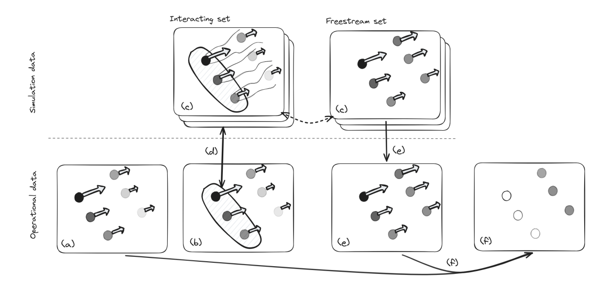
SCADA data is also used to estimate an operational wake loss time series, independently of the wake models. Tipspeed has developed a method suited to both onshore and offshore conditions (Davoust & Delaunay, 2025b), building on a previously published procedure (Nygaard et al., 2022). Starting from the 10-minute time series, the principle is to determine a freestream state for each turbine:

• Freestream turbine identification — at each timestep, turbines are classified as freestream when the ratio of their wind speed to the freestream wind speed exceeds a threshold (e.g. 0.995). If fewer than a minimum number qualify, the turbines with the highest ratios are added to ensure coverage.
• Site-specific simulations — two simulation sets are prepared for site-representative flow conditions: one assuming isolated turbines, one accounting for wake and blockage effects.
• Operational data matching — for each timestep, the closest matches in the interacting simulation set are found by comparing the power of freestream turbines in the operational data against the simulated values, using a Euclidean distance that keeps wind direction and power output similar.
• Freestream power estimation — the matched rows locate their counterparts in the isolated simulation set, and freestream power is estimated as the average power of those neighbours.
• Power deficit calculation — interaction losses are the difference between operational and freestream power. The steps are iterated to refine the site-specific simulations from the resulting wake deficit estimates.

Operational wake loss estimation. Top row: simulation datasets. Bottom row: operational data at a single timestep. (a) Pre-processing operational data. (b) Identifying freestream turbines. (c) Preparing site-specific simulations. (d) Matching operational data to simulations. (e) Estimating freestream power. (f) Calculating power deficits to freestream.

Actual power curve estimation

The actual power curve of each turbine is estimated by calibrating the wind speed input of the digital twin power model so that simulated power matches observed SCADA power.

Initial power comparison, before calibration.

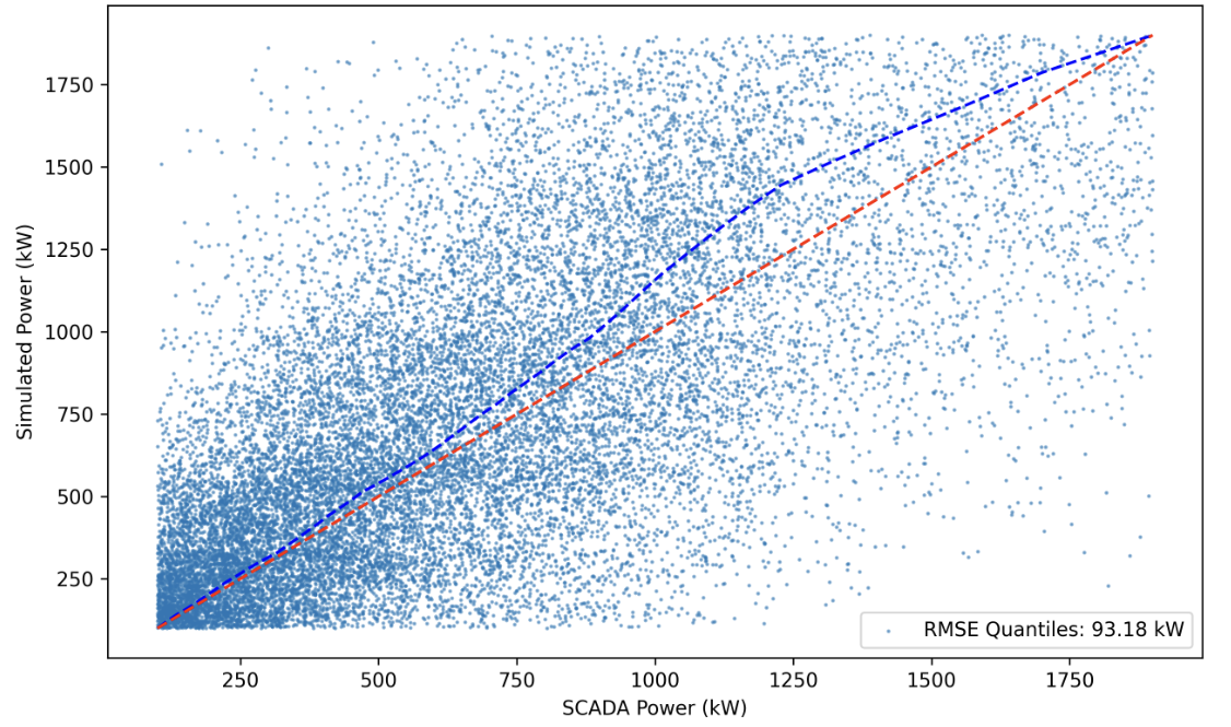
The calibration is quantile-based and uses only full performance operation. For each turbine, the power distributions of the two datasets are compared across quantiles (0%, 2%, 4%, …, 100%), and a spline model determines the wind speed adjustment required at each quantile to align simulated power with observed power. The correction captures turbine-specific performance characteristics that the reference power curve does not carry, and is validated by recalculating power with the adjusted wind speeds.

Final power comparison, after wind speed correction.

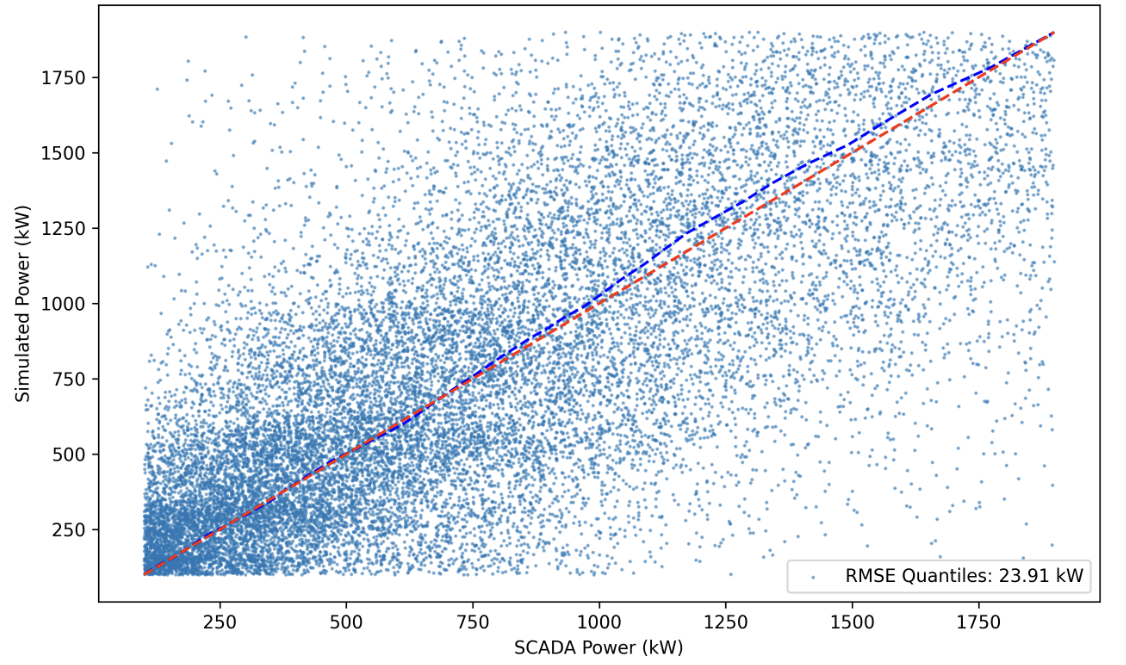
This improves the accuracy of the twin's power predictions by accounting for site- and turbine-specific performance, and provides a baseline for performance drift monitoring.

Upgrade analysis

Compares a Test group of turbines against a Control group over the same months, to separate what an upgrade did from what the weather did.

Only 10-minute rows where a turbine's SCADA status is full performance are used, which removes stops, curtailment and out-of-environmental-spec operation — none of which an upgrade causes, and all of which would otherwise dominate a monthly energy total. Over those rows, each group's measured energy is summed and divided by the Tipspeed-optimized expectation for the same rows:

\[\text{relative difference} = \left (\frac{\sum E_\text{SCADA}}{\sum E_\text{Tipspeed}} - 1\right) \times 100\]

The headline is the difference of the two groups' relative differences, in percentage points. Because each group is first compared against its own expectation, a windy month lifts both sides and cancels.

A month counts only when both groups have enough data: the group's full-performance 10-minute slots, divided by the whole calendar month (days × 144) times the number of turbines in the group, must reach the chosen minimum. The denominator is the whole month even when the selected date range cuts it, so a partial month at either edge falls below the threshold rather than appearing as a dip.

Energies are shown per turbine — each group's total divided by the number of turbines selected into it — so groups of different sizes are directly comparable.