Digital twin
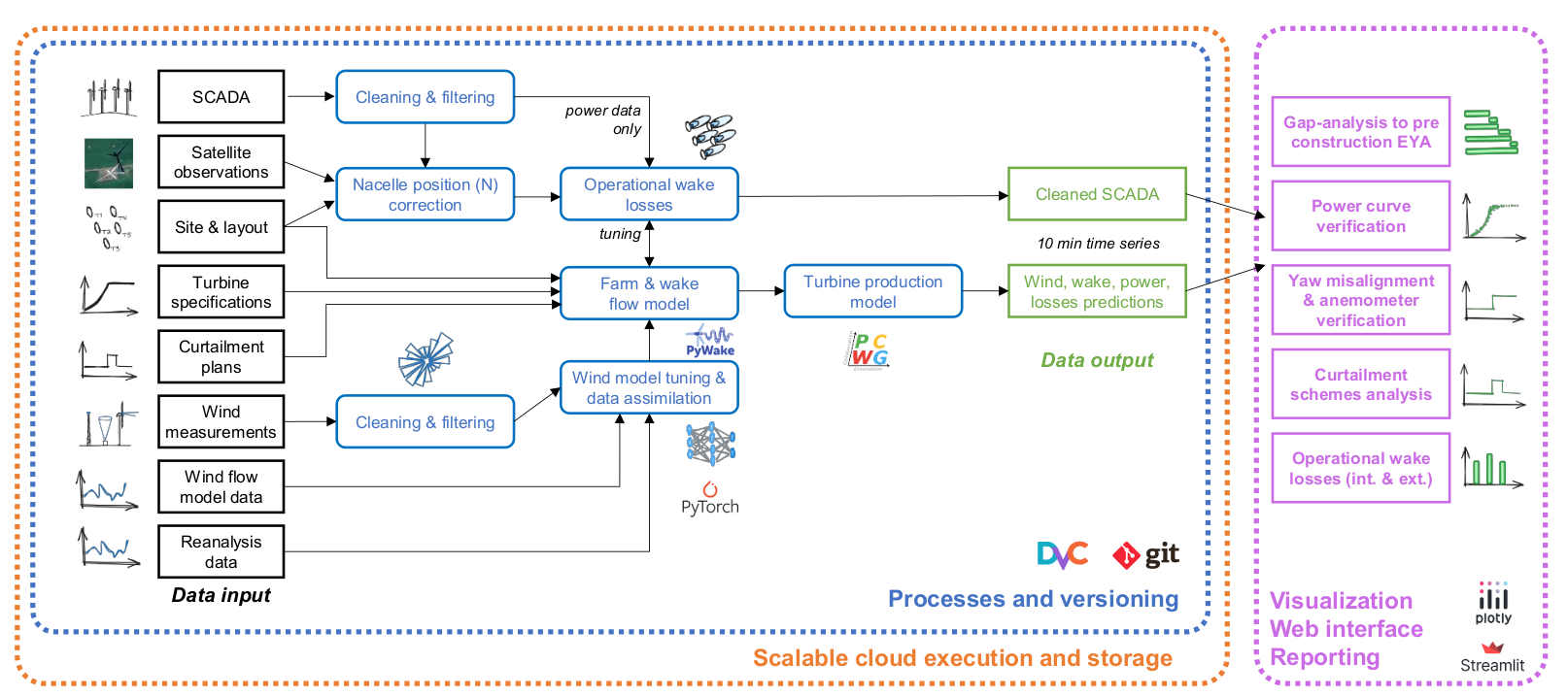
Tipspeed analyses wind farm performance by comparing operational data from the assets against independent reference data produced by a physics-based digital twin augmented with observations. The comparison is made turbine by turbine on 10-minute time series, which is what makes it possible to identify sources of underperformance — yaw misalignment, degraded power performance, availability — and to quantify the improvement potential of each.
The twin is built on three layers of physics-based models: a wind flow model, a wakes and blockage model, and a turbine performance model. Each layer is tuned and calibrated against a broad range of data sources: the site layout and reference power curves configure the simulation, pre-construction and operational wind measurements calibrate the wind flow model, satellite observations resolve turbine orientation, and operational data refines the wake and blockage models.
The approach is detailed in previous publications (Davoust, 2024a), (Davoust, 2024b) and (Davoust & Delaunay, 2025a), where the methodology was validated against 18 wind speed measurements across six different sites.
Wind flow
Physics model
An atmospheric Large Eddy Simulation (LES) numerical weather model is set up and executed over a domain covering the site, with a horizontal resolution of 100 m and a vertical resolution of 25 m. Its boundary conditions come from a mesoscale model covering an area of 250 km × 250 km, itself initialised from ERA5 reanalysis data. A surrogate model is then derived from the LES results to allow efficient spatial and temporal interpolation across the site.
Calibration and data assimilation
Tipspeed has developed a range of calibration and data assimilation methods that improve the accuracy of the wind flow model according to the reference data available for the site. They are organised in five levels:
| Level | Method | Added at this level |
|---|---|---|
| 0 | Pre-construction model | Calibration on pre-construction wind data |
| 1 | Wake calibration using SCADA data | Calibration on SCADA data (wake tuning) |
| 2 | Synchronisation using SCADA data | Time synchronisation with SCADA data |
| 3 | Calibration and synchronisation using wind measurements | Calibration on operational wind data |
| 4 | Assimilation of wind measurements | Assimilation of operational wind data |
Each level includes everything from the levels below it.
Wind direction offset calibration
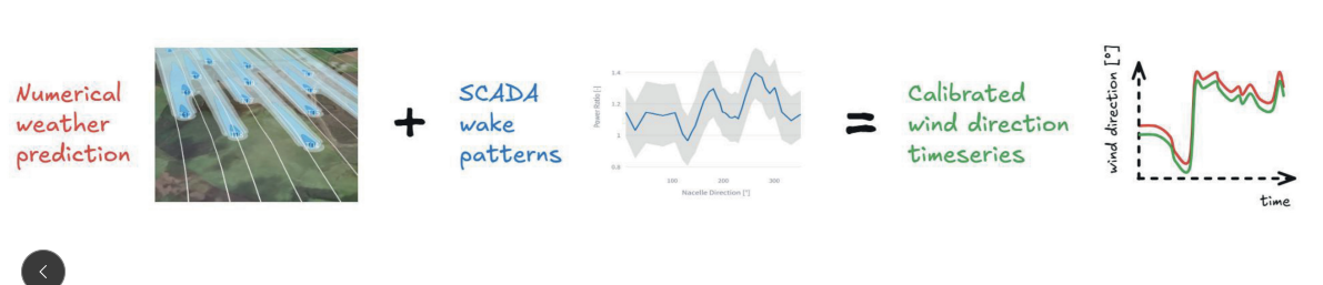
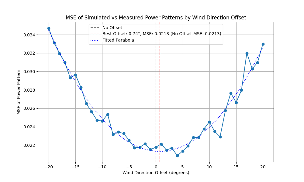
The wind direction produced by the model may deviate from the true direction by several degrees. It is finely calibrated by comparing the wake patterns observed in SCADA data with those predicted by the wake model: the simulated wind direction is shifted until both patterns align optimally.
Wakes and blockage
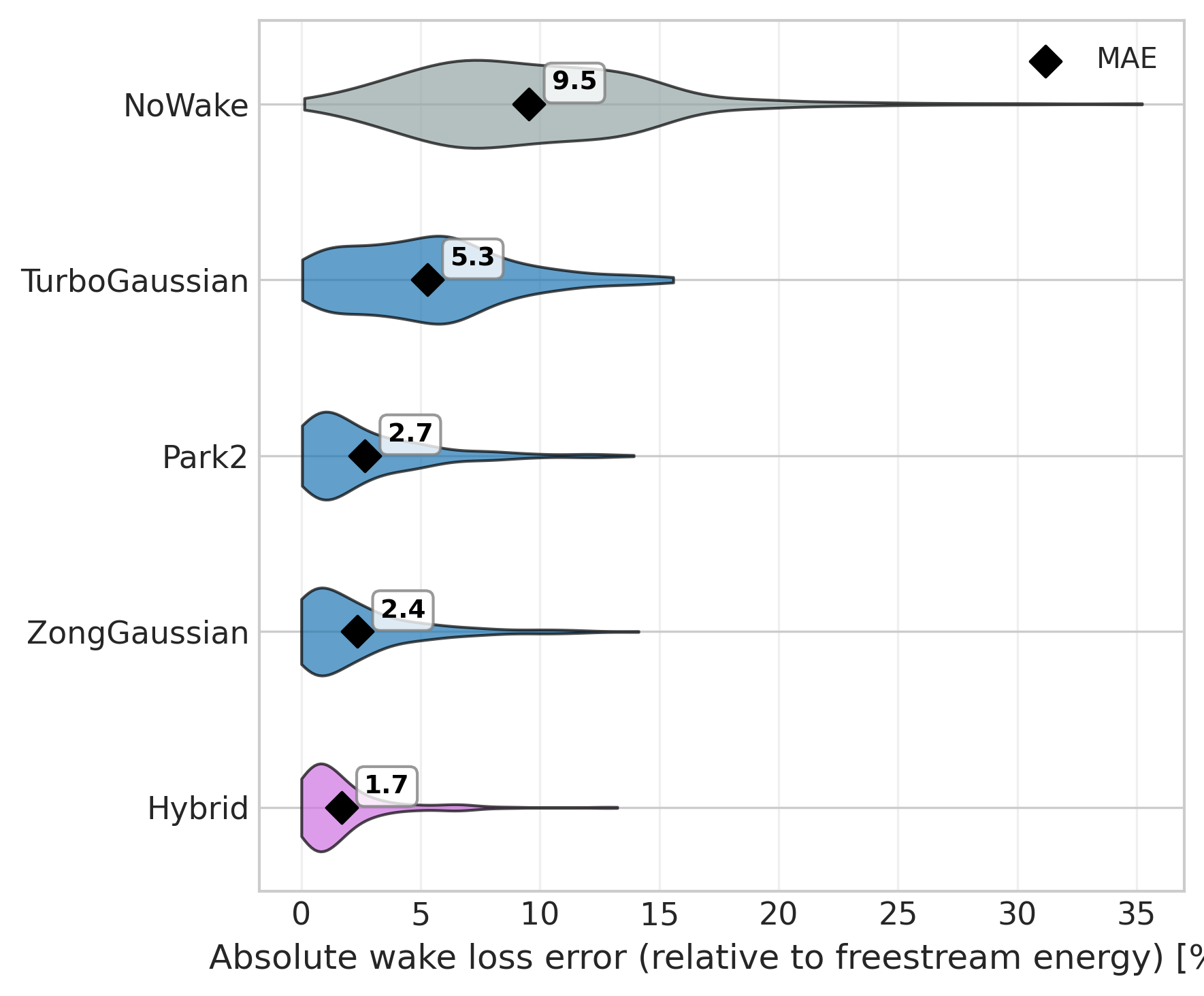
Wake and blockage losses are evaluated on 10-minute time series over the analysis period with PyWake (Pedersen et al., 2019). Wake modeling uses an ensemble of models: the TurbOPark Gaussian model (Nygaard et al., 2020), the Park2 model (Rathmann et al., 2018) and the Zong Gaussian model (Zong & Porté-Agel, 2020). Wind farm and turbine blockage is modeled by combining the wake deficit model with the scaled Rathmann blockage model (Meyer Forsting et al., 2021), and wake-induced turbulence with the Crespo–Hernández model (Crespo & Hernández, 1996).
Tipspeed validates wake models across all its projects (Davoust & Delaunay, 2026), which allows the best option to be selected for each site. The selected model is then tuned against operational data, as described below — this is the method used in delivered analyses.
Wake model parameter tuning
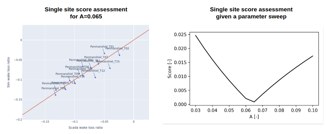
Wake model parameters are optimised per site against operational data, by minimising the error between the operational wake losses estimated from SCADA data (see Operational wake losses) and the wake losses predicted by the digital twin. The optimum is selected by grid search over the parameter space (Davoust & Delaunay, 2025b).
Hybrid wake modeling — research
Beyond the tuning above, Tipspeed is researching a hybrid wake model that uses machine learning to weight several engineering models so that they jointly best represent the observed wake losses. The benchmark above suggests it outperforms any single model, but it is a research avenue, not part of the delivered analyses: production results use the site-tuned single wake model described above.
A publication detailing the method is in preparation (Davoust & Delaunay, 2026); Tipspeed is happy to share preliminary results on request.
Turbine performance
Turbine performance is based on the reference power curves. Wind speed is normalised for air density on a 10-minute basis, following the IEC 61400-12-1 standard method (IEC, 2017).
Two further models establish the power deviation caused by turbulence intensity and by non-standard wind profiles. Both are adapted from IEC 61400-12-1, with empirical corrections that account for the real-life power response of turbines to wind (Davoust, 2018), and are validated at scale against field data (Davoust, 2026).
Why the standard corrections are tuned
Turbulence intensity, wind shear, upflow and veer across the rotor plane can cost several percent of production, yet these site-specific performance losses are rarely validated. The Power Curve Working Group established that the IEC 61400-12-1 adjustments for rotor equivalent wind speed (REWS) and hub-height turbulence intensity do not consistently reduce the variation of measured performance across atmospheric conditions (Davoust, 2018).
The common industry answer is a power deviation matrix derived from power curve tests. Those matrices rest on limited, proprietary datasets and may not generalise outside the conditions tested — least of all for larger turbines, which are more sensitive to these effects and less represented in the existing data.
Tipspeed instead adjusts the physics of the two IEC methods, as described below, and validates the result on operational data across its project fleet (Davoust, 2026).
Tuned rotor effective wind speed
IEC 61400-12-1 defines a rotor effective wind speed (REWS) correction for non-standard wind profiles. It extends first principles to non-homogeneous flow, assuming the turbine extracts energy according to the average of the cubed wind speed across the rotor disk.
Each turbine, however, has its own ability to convert a wind profile into power — it depends, among other things, on how the blade sections contribute to production. Tipspeed therefore tunes the REWS correction, minimising the error between observed power and the power predicted from the REWS-corrected wind speed.
The method computes a profile correction factor \( f \):
where:
- \( H_1 \), \( H_2 \) are the lower and upper bounds of the rotor disk
- \( l(z) \) is the rotor area weighting function at height \( z \)
- \( \alpha(z) \) is the upflow angle at height \( z \)
- \( \phi(z) \) is the wind direction veer deviation angle at height \( z \)
- \( v(z) \) is the wind speed at height \( z \), and \( v(z_0) \) the reference wind speed at the reference height \( z_0 \)
- \( n \) is an empirical exponent, tuned per turbine type
The factor is evaluated both on the measured profile (\( f_{meas} \)) and on a reference profile (\( f_{ref} \), a power law with a fixed exponent). The corrected wind speed \( v^{n} \) is then:
Tuned turbulence intensity correction
IEC 61400-12-1 also defines a correction of the power curve for non-standard turbulence intensity (TI). The standard method models the effect of turbulence by averaging a 0% TI steady-state power curve over the distribution of instantaneous wind speeds, which assumes the turbine tracks and responds to every turbulence scale measured at hub height:
where \( P_{est,meas}(TI) \) and \( P_{est,ref}(TI) \) are the expected power under measured and reference turbulence conditions.
That assumption does not fully capture turbine behaviour. Small turbulence scales are not spatially correlated across the rotor disk and are averaged out by the rotor's spatial extent, so the turbulence intensity that actually drives the power response is lower than the point measurement at hub height.
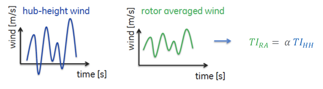
Tipspeed's tuned correction introduces a rotor-averaged turbulence intensity \( TI_{RA} \), derived from the hub-height measurement \( TI_{HH} \) through an empirical scaling factor \( \alpha \) (typically \( \alpha < 1 \)):
and applies the power correction with it:
\( \alpha \) is calibrated per turbine type by minimising the residual power performance variation across atmospheric stability conditions, which accounts for the rotor geometry, size and control system response of each turbine model.
Validation of the tuned corrections
The tuned REWS and TI corrections are validated by applying them to a wind farm digital twin and comparing against SCADA. The validation checks the consistency of power curves derived from daytime and nighttime conditions, which differ markedly in atmospheric stability and turbulence.
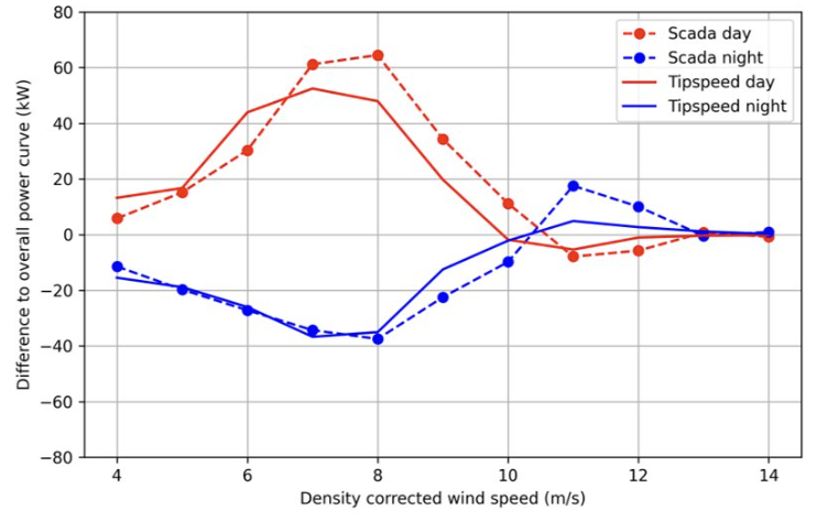
The corrections have also been validated at scale, across 11 sites and 334 turbines — two of the sites offshore — over 1.55 million freestream, normal-operation SCADA timestamps (Davoust, 2026). The validation targets power residuals, the deviation of each 10-minute point from the mean power curve trend, with the datasets normalised by rated power and rated wind speed so that turbines of different sizes can be compared. Observed residuals span −10% to +10% of rated power, with wind speed and turbulence intensity trends consistent with power performance tests; the model reproduces them with a correlation of 0.78 and virtually no bias — below 0.15% of rated power.
Long term and representative period
Annual production is dominated by how windy the year happened to be. Comparing one period against another — or one farm against another — therefore requires a common climate reference. Tipspeed builds one, and expresses results on both a representative period (long-term climate) and the current period (the actual analysis window), with an explicit windiness step between the two.
Long-term wind reconstruction
A machine learning model correlates an ensemble of multi-decade reanalysis and mesoscale sources — including ERA5 — against the site's own inflow, as measured on site and as simulated by the wind flow model. The model is trained over a window where both are available, then used to reconstruct the site inflow across the full history of the reanalysis sources, typically more than fifteen years.
Representative period
From that long-term history, a representative period is assembled: for each calendar day of the analysis window, one source day is drawn at random among all the years available for that same calendar day, and its 10-minute data is placed on the analysis calendar. Year-to-year variability is removed, while the seasonal and diurnal cycles of the site are preserved.
The pool of candidate days and the output window are independent: a climatology built from whole calendar years can be projected onto an analysis window that extends beyond it.
The representative inflow is then run through the same wake and turbine performance models as the rest of the twin, producing the Tipspeed long-term time series — expected production for an optimized farm, given a climate representative of the long term conditions (see Timeseries models).
Use in the energy chain
The energy waterfall starts on the representative period, at Gross (representative period), and walks to the current period through a windiness step — the difference between gross production over the representative period and over the current period. Because losses themselves depend on how windy the period was, site-specific performance and wake losses each carry their own windiness correction, computed as the difference between the current-period and representative-period value of that loss.
The result is a chain in which windiness is isolated in a single, explicit step, and every remaining step is a genuine performance effect. Definitions and formulas for each step are in the Metrics glossary.